Introduction
While preparing for my first multichannel piece I became aware of the need for more software tools designed in response to the kind of spatial thinking grown directly out of working with electroacoustic material (or at least electroacoustic as understood by a number of composers/researchers). In this respect, one of the least explored areas in multichannel software development is ‘circumspectral’ diffusion.
In his 2007 paper Space-form and the Acousmatic Image, Smalley refers to ‘circumspectral spaces’ as resulting from the combination of ‘spectral space’ and ‘circumspace’ - i.e. how the spectral content of a sound is distributed within the listening space to create a sense of ‘spatial scale and volume’[1]. As he elaborates:
How spectral space in itself is distributed contributes to the sensation of height, depth, and spatial scale and volume. I can create a more vivid sense of the physical volume of space by creating what I shall call circumspectral spaces, where the spectral space of what is perceived as a coherent or unified morphology is split and distributed spatially [2].
He goes on to discuss the concept in relation to his own compositions:
In my music, for example, circumspectral approaches have been particularly effective in imparting spatial volume to attack-resonance spectromorphologies, both to the attack phase and to prolonged, fluctuating, resonance-based forms, giving the impression that the listener is inside the resonance [3].
I. Background: Spectral Space
My research and compositional activities have for the most part been focused around the concept of spectral space - i.e. the impression of spatiality as attributed to the continuum of spectral frequencies [4]. Needless to mention that spectral space is not always pertinent to the listening experience. For instance, with clearly recognisable sound sources, the experience of spectral spatiality, which has a strong vertical bias, seems to be pushed into the background and instead one becomes aware of the suggested spatial settings of the sources themselves (i.e. ‘source-bonded’ spaces [5]). In general, sounds without direct extrinsic references encourage the listener to follow the spectromorphological attributes more closely: shapes and contours that articulate the domain of spectral frequencies. In this context the mental representation of ‘source’ and spectromorphology converge and spectral domain takes on spatial characteristics in our listening imagination: it becomes the dimension that is occupied by sound-shapes. Nevertheless, this does not suggest that spectral spatiality is divorced from source-bonded spaces. In a sense, spectral space can be seen as a schema abstracted from certain types of source-bonded spaces. Perhaps the vertical spatiality of the spectral domain is heightened by spectral and morphological characteristics that bear similarities with ecologically familiar sources - e.g. a high-frequency sound made up of short morphological units may evoke the utterance or [on a transmodal level] visual behaviour of smaller, sky-bound creatures. A striking example of this source-bonded nature of spectral space can be seen in the coda section of Risset’s Songes (starting at 6’.40”), where spectral space is reduced to its bare skeletal frame - a low, sustained drone supporting more animated higher frequency materials [6]. The spectral and perspectival motion of the higher material, coupled with its intrinsic spectral structure and morphology, clearly outlines a sort of birdlike flight or drift. Thus source-bonded, perspectival and spectral spaces work together to create a more vivid sense of spatial height and depth.
More on Circumspectral Space
In light of the above, my compositional interest in circumspectral sound diffusion is obvious. A similar method is used in certain diffusion systems where different types of loudspeakers are used for their characteristic sound quality (e.g. GRM’s Acousmonium) [7]. I have often diffused my works on loudspeaker orchestras that included overhead speakers. The signal is often passed through a high-pass filter before being routed into the overhead speakers. This allows one to exaggerate the sense of elevation in sounds that are already somehow elevated due to their spectral space occupancy and/or source-bonded characteristics. Naturally in a multichannel context one has far more control over the perspectival distribution of the spectral content during the composition stage. Although with careful mixing (e.g. in a DAW) one can certainly explore circumspectral spaces, it seem more appropriate to take advantage of a powerful audio-programming software like Csound to reduce the manual labour involved in such a task, whilst increasing the level of control offered to the composer. Ultimately, the intention is to create an environment that allows one to play with the ‘sculpting’ of spectra in circumspace in an intuitive and creative fashion.
On Reflection
Before explaining the Csound code and giving an overview of the Max/msp interface we must consider further consequences of the tool imagined above.
Firstly, the conventional notion of ‘spatialisation’ of a source within listening space is not strictly relevant here. Circumspectral diffusion involves the distribution of the spectral content of a unified spectromorphology - i.e. spreading the spectrum of a uniform sound (not to use the term ‘source’) in space, be it a single ‘figure’, a complex texture, or a combination of the two. Consequently, circumspectral panning is not used to position or move single sources around the audience; to a certain extent the aesthetic attitude that leads to the concept of circumspectral space (as defined by Smalley) contradicts the notion of spatial composition as arbitrary circumspatial positioning and movement of input sounds. In circumspectral diffusion, perspectival space becomes subordinate to spectral space, or rather, perspectival space is utilised to enhance the intrinsic spatiality of the sonic material - in this sense space is not seen as an empty canvas or container, but as an intrinsic quality inherent in the material.
Furthermore, perspectival motion-trajectories are automatically formed as a result of temporally stable distribution of spectral content of a sound that is itself characterised by dramatic spectral motion. To test this idea we can imagine that the frequency continuum is mapped onto the circumspatial domain defined by an array of loudspeakers, in such a way that the lower frequencies in the input sound are ‘panned’ at 0° and the increasing frequencies are contiguously arranged in a clockwise circular fashion around the listener. So the very highest frequency (e.g. 20kHz) takes us back to 0° in a full clockwise circle. In this case, a test sine-tone that glissandos from 20Hz to 20kHz will circle the listener in a clockwise fashion and finally terminate at 0° ‘position’ - a typical circular panning motion without any actual automation as shown in figure 1[8]!
Interesting circumspectral settings can be created by using complex spectromorphologies and creating a less straightforward circumspatial mapping of the spectral components. I have for instance had interesting results from noise-based sounds that were processed with numerous filter-sweep-like transformations to create broad spectral undulations. Even more interestingly, one can use stereo input sounds where the filtering motion is coupled with panoramic trajectories in the original stereo input. The stereo sound can then be mapped to the loudspeaker array as displayed above (the blue and red circles represent respectively the left and right channels of the input audio).
Note that the spectrum-to-circumspace mapping may be linear or logarithmic, the latter is perhaps more appropriate as the ear’s response to frequency increase and decrease is logarithmic. The above arrangement, used with the right sound material could lead to rather interesting spatio-morphological results in which the stereo image of the input sound is extended to a circumspatial image. Naturally the very lowest frequencies can seldom be localised so it would perhaps be more logical for the system to ignore the very lowest spectral frequencies (they can be mixed equally amongst the speakers) or even better, one could manually define the circumspectral mapping for each input sound - e.g. the most prominent spectral region in the sound can be panned to the front as to part-maintain the essence of the original stereo image.
II. Implementation
Concerning Sound Quality
The
flexibility of the pvs spectral processing opcodes in Csound have proven useful
to me in the past, so this seemed like the best place to start in order to
implement the aforementioned system. However, a note of warning must be included
here. By its very nature, the faithful reproduction of an original signal from
the data obtained by an FFT algorithm (as is the case with Csound’s pvanal
and pvsynth) requires all the analysed FFT bins (each bin represents a very
narrow frequency band). The omission or modification of the bins’ amplitudes
and/or frequencies will introduce more or less noticeable artefacts (i.e. phase-related
distortions), depending on the extent and nature of the modifications.
In this case we shall be using amplitude panning of the individual FFT bins and therefore artefacts will be introduced into the output signal as the bins become segregated and distributed amongst different speakers. (This implies the zeroing or attenuation of certain bins in different speakers - note that the bins exactly halfway between two speakers are mixed equally amongst two speakers.)
Optimal result is produced when no panning takes place and all the bins [from one input audio channel] are sent to one speaker. Obviously this defeats the point of implementing such a tool so we can minimise the unwanted artefacts by creating contiguous panning of the bins - the interface must encourage the user to make sure that the adjacent frequency bins are not drastically separated from each other in terms of their distribution amongst the loudspeakers. The random scattering of the bins within the circumspatial domain results in sounds with highly blurred transients (produced due to phase distortions), this may not be a problem for sustained morphologies but it will certainly be undesirable for transient materials. Using a hypothetical number of 16 bins, the right-side of the above scenario will produce audible artefacts (blurring, added resonance or AM-like ringing) as the bins are drastically scattered within listening space, whereas the left-side will produce an acceptable result, even for more transient sounds as shown above in figure 2.
Summary
In short, the algorithm works in the following steps:
- the input sound of each audio channel is analysed using
pvsanal - the resulting data for each analysis window is written to two tables (using
pvsftw), one for frequency and one for amplitude. Each table index contains the amplitude or frequency for one analysis bin. - the amplitude table is then passed unto a UDO, which recursively mixes the amplitude value for each bin among 6 tables (one for each loudspeaker), according to a 'panning' table that contains one panning value for each FFT bin at each index.
- the resulting 6 tables containing the amplitude values are then read frame-by-frame and coupled with the original frequency values (we do not alter the frequencies). The product is written into a
fsigstream (usingpvsftr). - finally the 6 output
fsigstreams are re-synthesised and routed into the appropriate speakers.
Implementation Part I
The pvsftr opcode used to write
the table data to an fsig stream requires an existing fsig stream.
Pvsinit may seem like an obvious choice here but in fact this opcode does not
update
the analysis frames, this would make the instrument dysfunctional [9].
A workaround is to use the pvsmix opcode to duplicate the fsig into
5 additional copies. These will later be overwritten by pvsftr so
the exact content does not matter, as long as the fsig formats
are identical. A simple resynthesis of the six fsig
streams at this stage would give six identical outputs, naturally not the desired
result.
ain1, ain2, ain3, ain4, ain5, ain6 inh 	;get input

			denorm  ain1 ;denormalise
fin1 pvsanal ain1,ifftsize,ihop,iwindow,iwindtype
;initialise remaining fsigs
fin2 pvsmix fin1, fin1
fin3 pvsmix fin1, fin1
fin4 pvsmix fin1, fin1
fin5 pvsmix fin1, fin1
fin6 pvsmix fin1, fin1
Next we must define the tables that are used to read and write the FFT data:
ifreqin1  ftgen 0,0,iNumBins,-2,0
iampin1   ftgen 0,0,iNumBins,-2,0
iampout1  ftgen 0,0,iNumBins,-2,0
iampout2  ftgen 0,0,iNumBins,-2,0
iampout3  ftgen 0,0,iNumBins,-2,0
iampout4  ftgen 0,0,iNumBins,-2,0
iampout5  ftgen 0,0,iNumBins,-2,0
iampout6  ftgen 0,0,iNumBins,-2,0
ifreqin1 is used to hold the frequency values that are common to all six resulting fsig streams (as we are not altering the frequencies directly).
iampin1 is used to hold the input amplitude values. And finally the iampoutN tables are used by the UDO to write the resulting mixed values in six separate locations.
Note that iNumBins, which defines the size of the ftables should be set to ifftsize/2+1 as defined at the top of the instrument (see csd).
In the interest of readability the names of the six output ftables (sited in the code snippet above) are passed to the UDO via a list held in a table:
iampoutlist ftgen 0,0,8,-2,iampout1, iampout2, iampout3, iampout4, iampout5, iampout6
Implementation Part II
We can also take advantage of the tabmorph opcode in the UDO
to have the possibility of morphing between two or more tables that hold the ‘panning’ values
for the FFT bins. The code snippet below defines four panning tables and two
control busses (the value of these busses are written from within the Max/msp
interface) for a two dimensional morphing plane that allows the user to morph
between the four tables.
kmorph_y	chnget "morph_y"
kmorph_x	chnget "morph_x"
kmorph_y	port	kmorph_y, 0.01, i(kmorph_y)
kmorph_x	port	kmorph_x, 0.01, i(kmorph_x)

;define 4 tables to be morphed
itabpan1    	ftgen 1,0,iNumBins,-7,1, iNumBins,1
itabpan2    	ftgen 2,0,iNumBins,-7,1, iNumBins,1
itabpan3    	ftgen 3,0,iNumBins,-7,1, iNumBins,1
itabpan4    	ftgen 4,0,iNumBins,-7,1, iNumBins,1

;pack them into a list
ipantablist     ftgen 0,0,4,-2,\
			itabpan1, itabpan2, itabpan3, itabpan4
Part III
Next we write the input fsig to the already
defined tables ifreqin1 and iampin1. Using the kflag output of pvsftw we ensure
that the table operations in the UDO is only activated when the frame has been
analysed and is ready for processing. Finally pvsftr is called six time to
access the six output tables (written inside the UDO mechanism) and transfer
their data into the predefined fsigs, before synthesising the result.
;engin
kflag0 pvsftw fin1, iampin1, ifreqin1
if (kflag0 > 0) then ; only proc when frame is ready

	circumspect	iNumBins, iampin1, ifreqin1,\
		iampoutlist, ipantablist, kmorph_x, kmorph_y

	pvsftr fin1, iampout1, ifreqin1
	pvsftr fin2, iampout2, ifreqin1
	pvsftr fin3, iampout3, ifreqin1
	pvsftr fin4, iampout4, ifreqin1
	pvsftr fin5, iampout5, ifreqin1
	pvsftr fin6, iampout6, ifreqin1
endif

;synthesise output
aout1 pvsynth fin1
aout2 pvsynth fin2
aout3 pvsynth fin3
aout4 pvsynth fin4
aout5 pvsynth fin5
aout6 pvsynth fin6

	outh	aout1, aout2, aout3, aout4, aout5, aout6
The User-Defined-Opcode
In principle the UDO
is rather simple. First we read the table names from iampoutlist and ipantablist
and ensure that the output tables are cleared before writing the calculated
bin values for the current frame.
iclear 		ftgen 0, 0, inumbins, -2, 0

;unpack list of ampout tables
iampout1	tab_i 0, iampoutlist
iampout2	tab_i 1, iampoutlist
iampout3	tab_i 2, iampoutlist
iampout4	tab_i 3, iampoutlist
iampout5	tab_i 4, iampoutlist
iampout6	tab_i 5, iampoutlist
;unpack list of pan tables
itab1		tab_i 0, ipantablist
itab2		tab_i 1, ipantablist
itab3		tab_i 2, ipantablist
itab4		tab_i 3, ipantablist

	;zero ampout tables before processing each frame
	tablecopy iampout1, iclear
	tablecopy iampout2, iclear
	tablecopy iampout3, iclear
	tablecopy iampout4, iclear
	tablecopy iampout5, iclear
	tablecopy iampout6, iclear
We also create
two temporary tables to hold the calculated morphed values for mixing the bins
among the six tables. These ‘buffer’ tables allow us to hold the
interpolated values between panning tables itab1, itab2 and itab3, itab4 and
further interpolate between them. Consequently, this gives us a two dimensional
morphing domain for morphing between four tables.
itabbuf1 	ftgen 0, 0, inumbins, -2, 0
itabbuf2 	ftgen 0, 0, inumbins, -2, 0
In the following section we recursively loop through the table indices (bin amplitude values) and the panning tables. After calculating the morphed panning value for the current bin, the input amplitude of the bin is read and mixed among six tables, depending on the panning value. The six speakers are treated in pairs so for instance when the panning value is 0.5 the bin is mixed equally between speakers one and two. A value of 1.5 means equal mixing between speakers two and three, and so on. Also note that we are using a constant power panning law with square root curve, which can be changed if desired.
kcount = 0
loop:
kout1	tabmorph kcount, kmorph_x, 0, 1, itab1, itab2
kout2	tabmorph kcount, kmorph_x, 0, 1, itab3, itab4
	tabw   kout1, kcount, itabbuf1
	tabw   kout2, kcount, itabbuf2

kpan	tabmorph kcount, kmorph_y, 0, 1,\
								itabbuf1,  itabbuf2
kamp		tab		 kcount, iampin

		if (kpan<=1) then
			kpan1 = sqrt(1-kpan)
			kpan2 = sqrt(kpan)
			tabw kamp*kpan1 , kcount, iampout1
			tabw kamp*kpan2 , kcount, iampout2
		elseif (kpan<=2) then
			kpan = kpan - 1
			kpan1 = sqrt(1-kpan)
			kpan2 = sqrt(kpan)
			tabw kamp*kpan1 , kcount, iampout2
			tabw kamp*kpan2 , kcount, iampout4
		elseif (kpan<=3) then
			kpan = kpan - 2
			kpan1 = sqrt(1-kpan)
			kpan2 = sqrt(kpan)
			tabw kamp*kpan1 , kcount, iampout4
			tabw kamp*kpan2 , kcount, iampout6
		elseif (kpan<=4) then
			kpan = kpan - 3
			kpan1 = sqrt(1-kpan)
			kpan2 = sqrt(kpan)
			tabw kamp*kpan1 , kcount, iampout6
			tabw kamp*kpan2 , kcount, iampout5
		elseif (kpan<=5) then
			kpan = kpan - 4
			kpan1 = sqrt(1-kpan)
			kpan2 = sqrt(kpan)
			tabw kamp*kpan1 , kcount, iampout5
			tabw kamp*kpan2 , kcount, iampout3
		elseif (kpan<=6) then
			kpan = kpan - 5
			kpan1 = sqrt(1-kpan)
			kpan2 = sqrt(kpan)
			tabw kamp*kpan1 , kcount, iampout3
			tabw kamp*kpan2 , kcount, iampout1
		endif

kcount = kcount + 1
if (kcount < (inumbins-1)) kgoto loop
Interface
A full description of the Max/MSP GUI is beyond the scope of this article so I shall limit myself to the basic principle here. The source-code is available for those interested in further exploration.
The instrument described above is used for only one input channel, but as mentioned before my intention was to be able to use stereo inputs. This is achieved from within Max/MSP by using two Csound~ objects, or rather two instances of Csound~ inside a poly~ object. The advantage of this method is that we can use two processors and achieve basic multithreading, one thread for each input channel [10]. Without this multithreading the instrument would be hardly usable in read-time due to the heavy duty UDO and the presence of six audio channels.
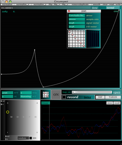
The interface uses a similar method as the GRM frequency warp plug-in described elsewhere [11] where the user can draw a function to fill the panning table. In this case the x axis denotes frequency and the y axis represents the panning value. The six speakers are mapped to values ranging from zero to six, where 0 = 6 (to allow a fully wrapped circle). The mapping can be linear or one of two alternative logarithmic scaling formulae (similar to the GRM tools interface) [12]. The user can define four such tables for the right and left channels each (eight in total) and morph between them with visual feedback. Copy and paste operations are allowed in-between the table so that the left and right input channels can be panned symmetrically if desired (see pp. 3-4). The interface, shown below in figure 3, is built to allow different configurations, for instance the output and input channels can be routed in any order, using a matrix object.
The user also has the option of filling the panning tables with statistically generated values, complete with masking functions, shown in figure 4. The values can be either scattered (to produce the aforementioned blurring effect) or smoothly interpolated (using a low pass filter for the statistical values).
III. Conclusion
The current circumspectral tool is far from complete, many more possibilities remain to be explored (e.g. using a vbap algorithm with a 3-D speaker array that includes overhead speakers). I hope that in this paper I have managed to encourage the reader to carry out further explorations of this uncharted territory. Perhaps one explanation for the rarity of such software tools is the relative absence of literature concerning spatial thinking in acousmatic music, particularly approached from an aesthetic point of view. The aousmatic space is manifold and is created through the interaction of spectral, percpectival and source-bonded spaces: circumspectral spaces are born as a facet of this interactive context. Moreover, not all sounds are open to all manners of spatial [perspectival] configurations - e.g. low frequency, sustained spectromorphologies cannot be used to create coherent spatial trajectories, on the other hand high frequency particles or textures beg for spatial animation and even evoke spatial trajectories without any actual perspectival motion. At a recent concert at Belfast’s SARC it was brought to my attention (by a non-musician) that some of the pieces included twisting and turning sounds that circled the audience or flew overhead. In fact these were all stereo pieces and even in the hands of a skilled diffuser the manual creation of circular percpectival motion would have been near-impossible. A clear indication that spectral motion alone can create the illusion of spatial motion.
All sounds occupy spectral space (which may or may not be perceptually pertinent, depending on the listening context) and all sounds suggest source-bonded spaces. Consequently, all sounds are by their very nature pregnant with an inherent spatiality. It is my view that there is far more to the composition of space [and spatial thinking in acousmatic music] than source-localisation and movement within listening space, often referred to as ‘spatialisation’. Although such technology is much needed and highly valuable for the acousmatic composer, from a compositional stance the notion of ‘spatialisation’ can potentially lead to a simplistic and sterile aesthetic approach that neglects the inherent spatiality of sounds - I prefer the terms ‘perspectival projection’ to ‘spatialisation’. It is the understanding of this inherent spatiality and our perception of it that must guide the composition of space in acousmatic music. One could even go as far as to suggest that it is the power to create spatiality that marks acousmatic music as a unique form of artistic expression. We need more technological tools and research that enrich our ability to explore and sculpt sonic spatiality in an aesthetically sophisticated manner.
References
[1]
D. Smalley, "Space-form and the Acousmatic Image", Orgnized Sound,
Volume 12, Issue 01, 2007, p. 51.
[2] Ibid., p. 51.
[3] Ibid., p. 51.
[4] Ibid., pp. 44-45.
[5] Ibid., p. 38.
[6] J.-C. Risset, Computer Music: Why?,
Available: http://www.utexas.edu/cola/insts/france-ut/_files/pdf/resources/risset_2.pdf.[Accessed 07/04/2011].
[7] H. Tutschku, On the Interpretation of Multi-Channel
Electroacoustic Works on Loudspeaker Orchestras. Available: http://www.tutschku.com/content/interpretation.en.php.[Accessed 07/04/2011].
[8] Note that the above paragraph serves only as an example and the writer
does not recommend it as a compositional device.
[9] Thanks to Victor Lazzarini for pointing this out to me
[10] This idea was originally suggested by Alexis Baskind.
[11] P. Khosravi, "Implementing Frequency Warping", Csound
Journal,
Issue 12, December 13, 2009. Available: http://www.csound.com/journal/issue12/implementingFrequencyWarping.html.
[12] I am very grateful to Alexis Baskind for assisting the implementation
of the logarithmic scaling of the graph.