Csound Journal

Introduction

In the old time of analog synthesizers, producing complex sounds was easy by connecting the audio output of one VCO to the frequency control input of another VCO and connecting the audio output of the latter to the frequency control input of the first one. This simple patch could yield a chaotic result as illustrated by Dan Slater [1]. Our article describes a Csound plugin presenting a few opcodes implementing such patches.

I. Overview

crossfm

The crossfm and crossfmi opcodes implement cross frequency modulation between two oscillators as shown in the following diagram:

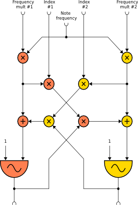
Figure 1. Diagram of the crossfm opcode.

The syntax is:

a1, a2 crossfm xfrq1, xfrq2, xndx1, xndx2, kcps, ifn1, ifn2 [, iphs1] [, iphs2]
a1, a2 crossfmi xfrq1, xfrq2, xndx1, xndx2, kcps, ifn1, ifn2 [, iphs1] [, iphs2]

where the parameters are:

xfrq1 -- a parameter that, when multiplied by the kcps parameter, gives the frequency of oscillator #1.
xfrq2 -- a parameter that, when multiplied by the kcps parameter, gives the frequency of oscillator #2.
xndx1 -- the index of the modulation of oscillator #2 by oscillator #1.
xndx2 -- the index of the modulation of oscillator #1 by oscillator #2.
kcps -- a common base value, in cycles per second, for both oscillator frequencies.
ifn1 -- function table number for oscillator #1 (usually a sinewave).
ifn2 -- function table number for oscillator #2 (usually a sinewave).
iphs1 (optional, default=0) -- initial phase of waveform in table ifn1, expressed as a fraction of a cycle (0 to 1). A negative value will cause phase initialization to be skipped.
iphs2 (optional, default=0) -- initial phase of waveform in table ifn2, expressed as a fraction of a cycle (0 to 1). A negative value will cause phase initialization to be skipped.

crossfmi behaves like crossfm except that linear interpolation is used for table lookup.

crosspm

The crosspm and crosspmi opcodes implement cross phase modulation between two oscillators as shown in the following diagram:

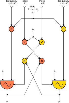
Figure 2. Diagram of the crosspm opcode.

The syntax is:

a1, a2 crosspm xfrq1, xfrq2, xndx1, xndx2, kcps, ifn1, ifn2 [, iphs1] [, iphs2]
a1, a2 crosspmi xfrq1, xfrq2, xndx1, xndx2, kcps, ifn1, ifn2 [, iphs1] [, iphs2]

where the parameters have the same meaning as in crossfm, and again crosspmi uses linear interpolation for table lookup.

crossfmpm

Finally, the crossfmpm and crossfmpmi opcodes implement cross frequency/phase modulation between two oscillators as shown in the following diagram:

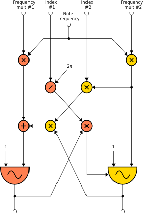
Figure 3. Diagram of the crossfmpm opcode.

The syntax is:

a1, a2 crossfmpm xfrq1, xfrq2, xndx1, xndx2, kcps, ifn1, ifn2 [, iphs1] [, iphs2]
a1, a2 crossfmpmi xfrq1, xfrq2, xndx1, xndx2, kcps, ifn1, ifn2 [, iphs1] [, iphs2]

where the parameters have the same meaning as in crossfm, and crossfmpmi and use linear interpolation for table lookup. Oscillator #1 is frequency-modulated by oscillator #2 while oscillator #2 is phase-modulated by oscillator #1.

II. Technical issues

Frequency modulation vs phase modulation

In frequency modulation, the frequency of the carrier is modified by the modulator while in phase modulation, it is the phase of the carrier that is modified. In single modulation, the audio result is the same with both modulations, even though the algorithms are different. On the other hand, if we introduce feedback loops like in the opcodes above, the audio result from frequency modulation will differ from the phase modulation one. This is due to the fact that each oscillator being modulated, their waveforms become complex and a dc component may appear in their spectra. This dc component may be considered as having a frequency of 0 Hz. If the oscillator is frequency modulated, this 0 Hz component will be shifted by the modulation like the other frequencies, thus becoming audible. Conversely, if the oscillator is phase modulated, the dc component will remain an inaudible dc component (a more detailed explanation is given in the article by Russel Pinkston in "The Csound Book" [2]).

In normal use, people often prefer phase modulation in order to avoid the annoyance of the dc shift, especially if the purpose is to mimic acoustic instruments as with the famous DX7 synthesizers by Yamaha in the 1980's. Here, on the contrary, we will take advantage of this feature in the cross frequency modulation.

Sampling rate

Usually, opcodes are supposed to operate in the same way, irrespective of the sampling rate value, with the only difference that a higher sampling rate yields a broader bandwidth and thus a better sound quality. In cross frequency modulation, we can have very rich spectra, especially with high modulation indexes, and in some cases foldover aliases may occur if the sampling rate is not high enough. Moreover with non-linear feedback loops a different sampling rate means a different step size in the algorithm difference equations and then a different audio result due to the non-linearity of the algorithm. In Csound, two other opcodes have the same characteristics: planet and chuap.

We can hear this in the following example: artefacts.ogg. Four notes are played by crossfm with the same parameters (frq1=517.505, frq2=735.696, ndx1=3, and ndx2=3) but increasing sampling rate (48kHz, 96kHz, 192kHz, and 384kHz).

When working with those opcodes, you should use a sampling rate as high as possible. If you need to produce a CD quality file, you should first produce a high sampling rate file and then downsample this file using the srconv utility, with a command like this:

srconv -Q 4 -r 44100 -W -s -o cdqualityfile.wav highsrfile.wav

The plugin source code

The plugin source code is given in this archive file. If you adapt the included Makefile to your environment, you can use it to build the plugin. More information about plugin opcodes is available at [4].

III. Exploring the parameter space

A GUI for testing

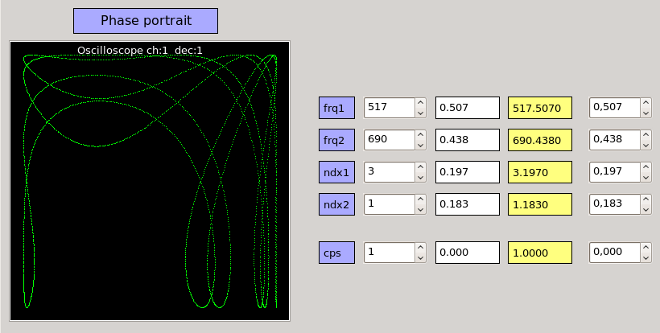
We can use Qutecsound ([3]) and its widget set to build a friendly GUI to explore the different values of the parameters. The oscilloscope widget was modified so that it can display Lissajou curves or Poincaré maps. This new feature is available in the version 0.4.5 of Qutecsound.

The cfmgui.csd file can be used as a testing GUI for crossfm. Each parameter can be set via a coarse value spin box for its integer part, a fine value scroll number and/or spin box for its decimal part. The stereo output of the instrument is displayed through the oscilloscope widget as a phase portrait (Lissajou curve mode):

Figure 4. Widget panel of cfmgui.csd in Qutecsound.

Automated exploration

Besides using the GUI described above to test the parameters, we can use interactive genetic algorithms as described by Colin G. Johnson [5]. Genetics algorithms are exploration tools based upon natural selection and genetics.

A population of individuals is randomly created. Each individual represents a set of parameters to control the orchestra for the generation of one single note. The parameters are concatenated into a "chromosome" as a binary string. Each individual receives a fitness value. Usually, this fitness value is calculated from an optimization function. Here, we use instead a set of sliders in a graphical interface to manually set the fitness value of each sound (this is the interactive part). A new generation is then processed by selecting individuals in the old generation in function of their fitness, recombination of the selected individuals (crossover) and mutation.

The "blue" frontend ([6]) with its scripting language Jython (a Java written version of Python) is a good candidate to implement a Simple Genetic Algorithm. The cfm_ga.blue file has a Score Timeline including four soundObjects. The first one is a Comment describing the project. The second one is a PythonObject implementing the classes of a Simple Genetic Algorithm as described in ([7]). The following diagram shows the classes:

Figure 5. Classes of the Simple Genetic Algorithm.

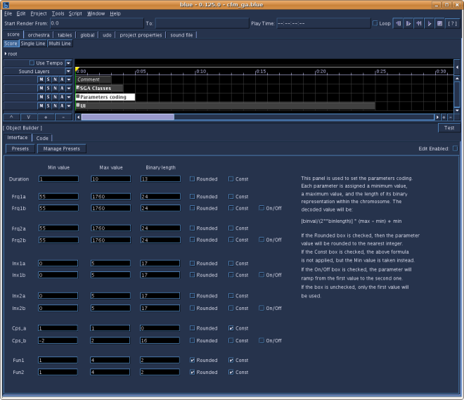
The third soundObject is an ObjectBuilder that displays an interface for the parameters coding. Each parameter is given min and max values and the number of bits of its binary coding within the binary string (chromosome). Some parameters have 'a' and 'b' entries. This means that if the 'b' entry is activated, the parameter value will ramp between the 'a' and 'b' values during the note length. The parameters are input arguments for one of the three orchestras; for example the crossfm test orchestra is:

idur      =         p3
iamp      =         p4
ifq1a     =         p5
ifq1b     =         p6
ifq2a     =         p7
ifq2b     =         p8
inx1a     =         p9
inx1b     =         p10
inx2a     =         p11
inx2b     =         p12
icpsa     =         p13
icpsb     =         p14
ifn1      =         p15
ifn2      =         p16
iphs1     =         p17
iphs2     =         p18
kfrq1     line      ifq1a, idur, ifq1b
kfrq2     line      ifq2a, idur, ifq2b
kndx1     line      inx1a, idur, inx1b
kndx2     line      inx2a, idur, inx2b
kcps      line      icpsa, idur, icpsb
kenv      linen     iamp, 0.05, idur, 0.2
a1, a2    crossfm   kfrq1, kfrq2, kndx1, kndx2, kcps, ifn1, ifn2, iphs1, iphs2
          outs      a1*kenv, a2*kenv

Figure 6. Parameters coding interface.

The fourth soundObject is an ObjectBuilder that displays the user interface (UI) for running the genetic algorithm.

Figure 7. User Interface.

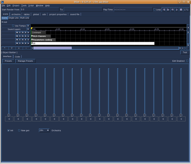
You first have to select the Parameters Coding soundObject and choose the settings you want. Then you select the UI soundObject. Each time you press the play button, one of three possibilities happens. If the Init box is checked, a new SGA is initiated with its first generation randomly calculated. If the Init box is unchecked and the New gen box is unchecked, you hear again the sounds of the last calculated generation. This is useful to set correctly the fitness values (slider controls). Finally, if the Init box is unchecked and the New gen box is checked, a new generation is calculated by the SGA depending on the fitness values set by the user.

Note: the first time you hit the play button, the Init box MUST be checked, otherwise you will get a Jython error. This is due to the fact that when you open the cfm_ga.blue file, the ga object does not exist within the Jython memory space, and the only way to create a new ga object is to hit the play button while the UI Init box is checked.

IV. Examples

The first example (ex01.csd) is a continuous sound with fixed frequencies, while the modulation indexes are moving along a ramp. To get more relief, the sound is granulated through instrument #2. (ex01.ogg)

The second example (ex02.csd) is a pseudo-melody with an exotic tuning that is obtained by varying the modulation indexes. The first note is played using two sine waves. The second note is played using two pseudo-square waves with the modulation indexes variation reversed: the "melody" seems played backwards and the timbre is richer. The third note is like the first one but it is two seconds longer and thus the "melody" is slower. The fourth note is like the second one, but with two sine waves, longer duration and the second frequency one Hz higher, giving a richer tremolo. (ex02.ogg)

The third example (ex03.csd) uses cross phase modulation to simulate an old airplane engine. The function table used is a pseudo-sawtooth waveform. Note that the Ogg Vorbis compression algorithm has changed the original sound. You should play the example from csound to hear the original sound. (ex03.ogg)

Conclusion

Csound is a powerful and ubiquitous software. In this article it has been shown how Csound can be used to build specific tools adapted for particular research. Thanks to the developers, rich frontends exist for Csound that allow us to rapidly test new ideas and build exploration tools. In 1963, the composer Iannis Xenakis wrote in the first French edition of his famous book "Musiques Formelles" ([8]): "With the aid of electronic computers the composer becomes a sort of pilot: he presses the buttons, introduces coordinates, and supervises the controls of a cosmic vessel sailing in the space of sound, across sonic constellations and galaxies that he could formerly glimpse only as a distant dream. Now he can explore them at his ease, seated in an armchair". In 1963 this type of writing could be considered visionary writing, but today it is a reality.

Acknowledgements

I want to thank Andrés Cabrera for giving me technical informations to modify the QuteCsound oscilloscope widget so that it could display Lissajou curves. Thanks to Steven Yi and to Victor Lazzarini for sending me references about frequency modulation and feedback oscillators. Finally I would like to thank the editors James Hearon and Steven Yi for giving me extra time to develop the genetic algorithms section.

References

[1] Dan Slater, Chaotic sound synthesis, Computer Music Journal 22 (2) (1998), 12-19.
[2] Russel Pinkston, FM Synthesis in Csound, The Csound Book (2000), The MIT Press, 261-279
[3] Andrés Cabrera, QuteCsound.
[4] Victor Lazzarini, Extensions to the Csound Language: from User-Defined to Plugin Opcodes and Beyond.
[5] Colin G. Johnson, Exploring the sound-space of synthesis algorithms using interactive genetic algorithms, Proceedings of the AISB workshop on artificial intelligence and musical creativity, 1999.
[6] Steven Yi, blue.
[7] David E. Goldberg, Genetic Algorithms, Addison-Wesley USA, (15767), 1991.
[8] Iannis Xenakis, FORMALIZED MUSIC: Thought and Mathematics in Music, Pendragon Revised Edition, Pendragon Press, 1992.